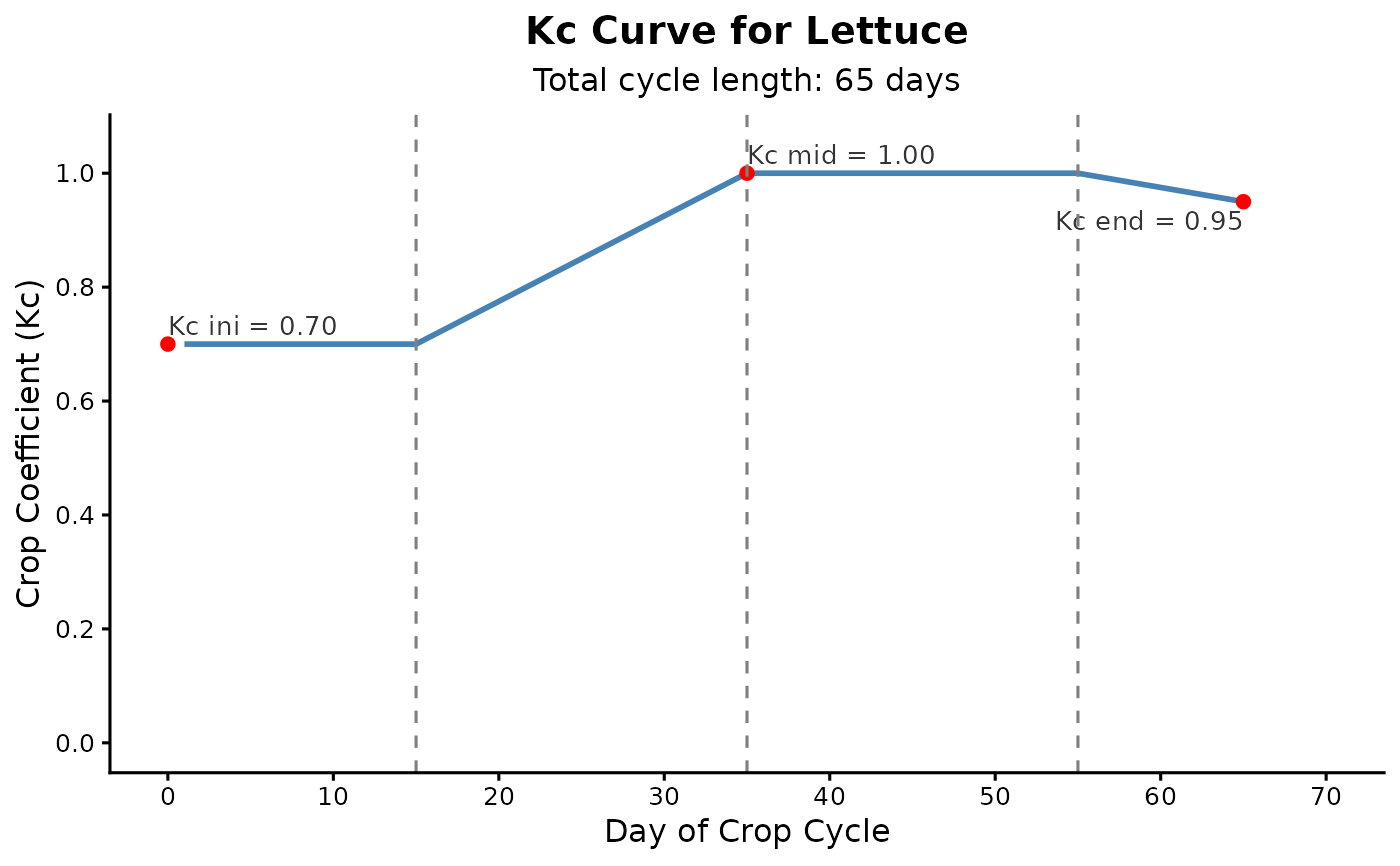
Constructs a time series of daily crop coefficient (Kc) values and generates a ggplot2
visualization representing the Kc curve over the crop cycle, following FAO-56 guidelines.
The curve is divided into four stages: initial, development, mid-season, and late-season.
Arguments
- kc_points
Numeric vector of length 3. Contains the crop coefficients for the initial stage (
Kc_ini), mid-season stage (Kc_mid), and end of the late-season stage (Kc_end).- stage_lengths
Numeric vector of length 4. The duration (in days) of each growth stage: initial, development, mid-season, and late-season.
- crop
Character (optional). Name of the crop, used to customize the plot title.
Value
A list containing:
kc_serie: A numeric vector of daily Kc values over the entire cycle.kc_plot: Aggplot2object displaying the constructed curve with key annotations.kc_data: A data frame containing the days and their corresponding Kc values.
References
Allen, R. G., Pereira, L. S., Raes, D., & Smith, M. (1998). Crop evapotranspiration - Guidelines for computing crop water requirements. FAO Irrigation and drainage paper 56.
Examples
kc_points <- kc_params_lettuce <- c(0.7, 1.0, 0.95) # Kc_ini, Kc_mid, Kc_end
stage_lengths <- stage_lengths_lettuce <- c(15, 20, 20, 10) # L_ini, L_dev, L_mid, L_late
lettuce_data <- calc_kc_curve(
  kc_points = kc_params_lettuce,
  stage_lengths = stage_lengths_lettuce,
  crop = "Lettuce"
)
print(lettuce_data$kc_data)
#>    day kc_value
#> 1    1    0.700
#> 2    2    0.700
#> 3    3    0.700
#> 4    4    0.700
#> 5    5    0.700
#> 6    6    0.700
#> 7    7    0.700
#> 8    8    0.700
#> 9    9    0.700
#> 10  10    0.700
#> 11  11    0.700
#> 12  12    0.700
#> 13  13    0.700
#> 14  14    0.700
#> 15  15    0.700
#> 16  16    0.715
#> 17  17    0.730
#> 18  18    0.745
#> 19  19    0.760
#> 20  20    0.775
#> 21  21    0.790
#> 22  22    0.805
#> 23  23    0.820
#> 24  24    0.835
#> 25  25    0.850
#> 26  26    0.865
#> 27  27    0.880
#> 28  28    0.895
#> 29  29    0.910
#> 30  30    0.925
#> 31  31    0.940
#> 32  32    0.955
#> 33  33    0.970
#> 34  34    0.985
#> 35  35    1.000
#> 36  36    1.000
#> 37  37    1.000
#> 38  38    1.000
#> 39  39    1.000
#> 40  40    1.000
#> 41  41    1.000
#> 42  42    1.000
#> 43  43    1.000
#> 44  44    1.000
#> 45  45    1.000
#> 46  46    1.000
#> 47  47    1.000
#> 48  48    1.000
#> 49  49    1.000
#> 50  50    1.000
#> 51  51    1.000
#> 52  52    1.000
#> 53  53    1.000
#> 54  54    1.000
#> 55  55    1.000
#> 56  56    0.995
#> 57  57    0.990
#> 58  58    0.985
#> 59  59    0.980
#> 60  60    0.975
#> 61  61    0.970
#> 62  62    0.965
#> 63  63    0.960
#> 64  64    0.955
#> 65  65    0.950
print(lettuce_data$kc_plot)